A point on Organisationational Drift
Time to wrap up the Audit 2.0 serie, and everything points to the fact that businesses do not go from healthy to broken, rather travel there, along a path, at a speed.

The whole serie about Auditing 2.0 was about leaving the idea we can tell when something breaks it would scatter from 0 to 1. All is about spotting risk of sustained march towards the pitfall: deviating from where healthy business and operations should go can be conceptualized as the subject of interest, the organization, operations control, is drifting away. What does it mean to drift? Not to fail, not to breach, not to trigger but to move. To be in transit between one distributional state and another, at some speed, along some path.
This post answers that question. It names the geometric object that formalises drift, shows where it lives, and reveals that every instrument we have built across this series was measuring the same thing from a different angle, through a different aperture, with a different degree of loss.
The unification is not a synthesis of five tools. It is the discovery that one object was always casting five shadows.
A Synthesy Diagram
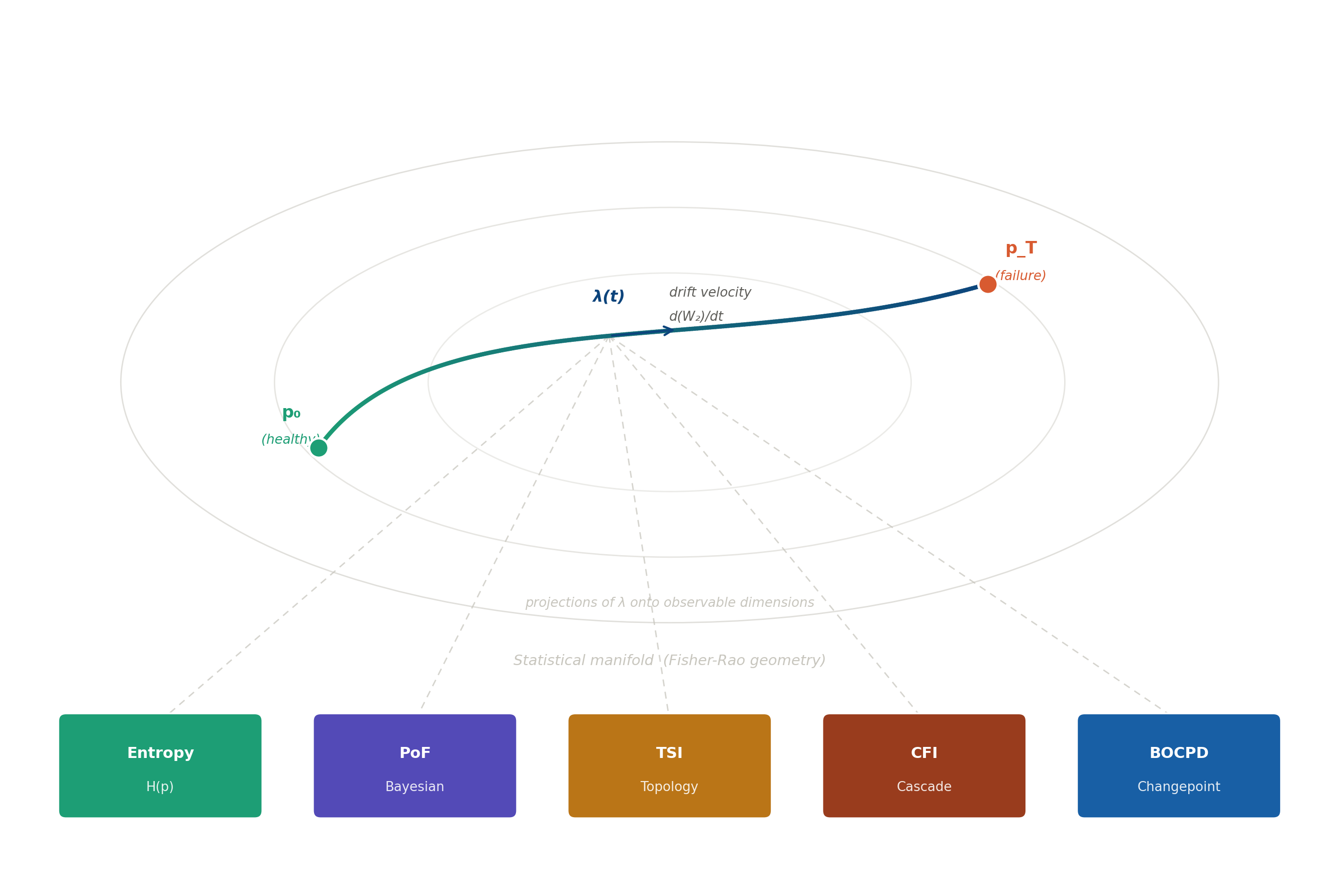
This is a geometric picture of what organisational failure looks like, before any threshold is crossed.
The nested ellipses are not decorative: they are the contour lines of the Fisher-Rao metric, the geometry of statistical distinguishability. Every point on this surface is a probability distribution. Every path through it is a trajectory of change. The blue curve is a real process travelling from its healthy baseline p₀ toward failure at p_T. The arrow mid-trajectory is λ(t), the drift velocity: not a metaphor but a derivative, a rate of change measured in the geometry of optimal transport.
The five coloured boxes at the bottom are the instruments of this series. The dashed lines connecting them to the trajectory are projections: each instrument catching the shadow of the same object from its own angle.
There is nothing missing from this picture. Everything we need is already here.
The object
When a process fails slowly, not catastrophically but incrementally, distributional state by distributional state, what is happening, in precise mathematical terms, is that the probability distribution governing the process is moving through the space of all distributions.
The mathematical object that measures the speed of that movement is the 2-Wasserstein distance: the Earth Mover’s Distance, the minimum cost of transporting one distribution into the other. For Gaussian distributions this reduces to something intuitive: the squared distance between two distributions is simply the squared difference in their means plus the squared difference in their standard deviations. The geometry is Euclidean in parameter space, with optimal transport as the underlying justification.
The drift velocity (call it λ) is simply the rate at which that Wasserstein distance grows over time. Not a threshold. Not a ratio. A speed, measured in the geometry of distributional change.
This is not a metaphor, as λ is a genuine velocity - the speed at which a process is moving away from where it should be.
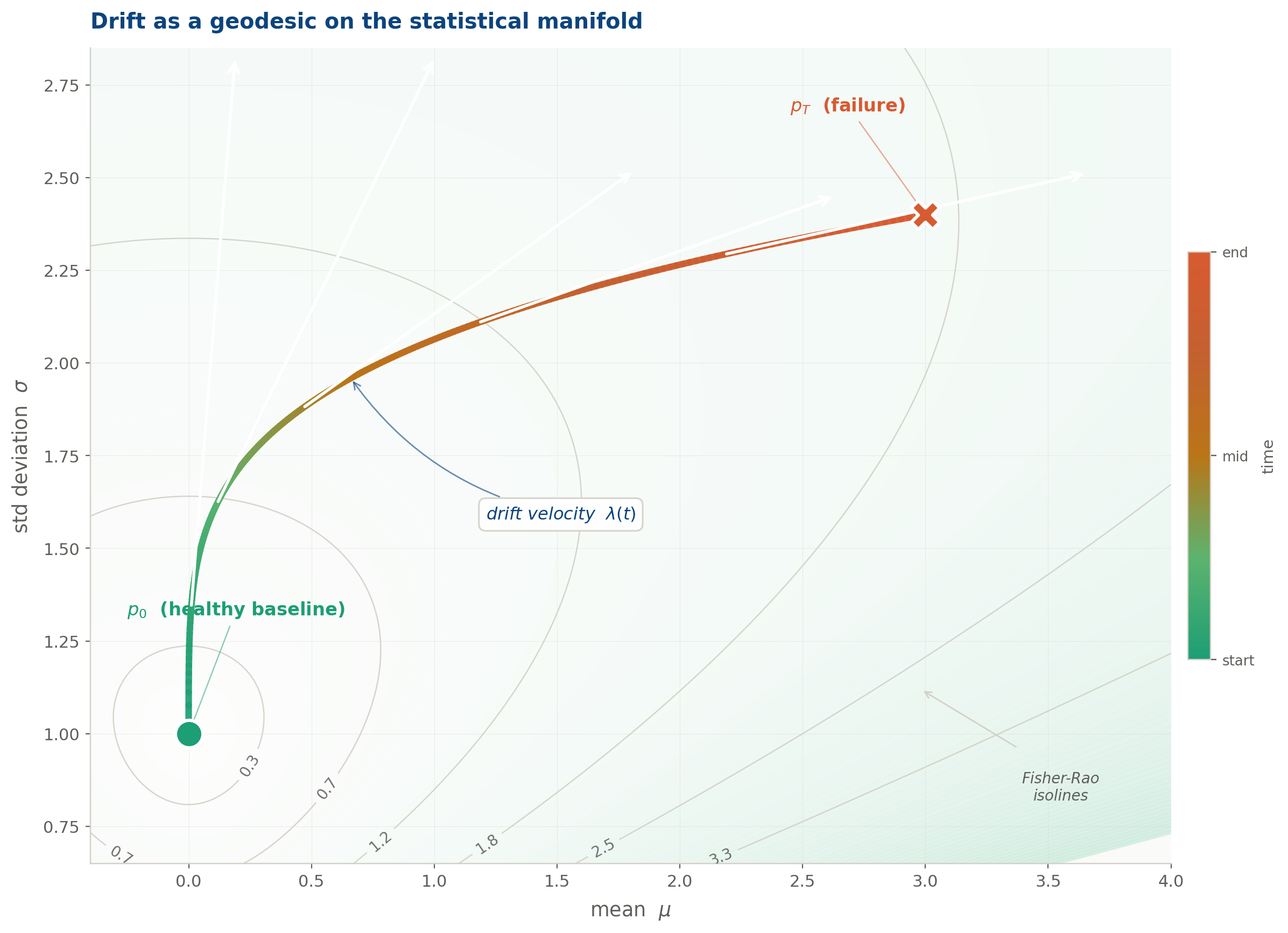
The drift trajectory plotted directly in (μ, σ) parameter space, the statistical manifold of the Gaussian family. The trajectory is colour-graded from teal (healthy baseline p₀) through amber to rose (failure state p_T). Fisher-Rao isolines show the geometry: each contour is a set of distributions at equal statistical distinguishability from p₀. The trajectory curves steeply at first as σ rises, then sweeps right as the mean accelerates. The white arrows show drift velocity at five points along the path.
The statistical manifold
The Wasserstein space tells us how far a distribution has travelled. But it does not tell us, in the most operationally useful sense, how fast it is becoming unrecognisable. For that, we need a different geometry: one that measures distance in units of statistical distinguishability rather than transport cost.
The Fisher information metric equips the space of parametric distributions with exactly this geometry. The Fisher information matrix encodes how much information a single observation carries about the parameters: how sharply the distribution responds to small changes in its description. Where the Fisher information is large, the geometry is curved: distributions in that region are highly distinguishable from their neighbours, and small parametric movements produce large statistical separations. Where it is small, the geometry is flat: the distribution is insensitive to perturbation, and change is hard to detect.
For the Gaussian family, the Fisher matrix gives different weights to mean drift and variance drift: specifically, variance drift is penalised more heavily, because changes in spread are statistically detectable at finer scales than changes in location. The resulting Fisher-Rao drift velocity combines both: mean drift scaled by how concentrated the distribution is, and variance drift scaled by the same factor but weighted twice as strongly.
That asymmetry is the key result of this section, and it has a direct practical consequence.
The sentence this series was building toward
A process drifting fast in Fisher-Rao terms is one whose output distributions are becoming rapidly distinguishable from their recent past, which is precisely what failure looks like, before any threshold is crossed.
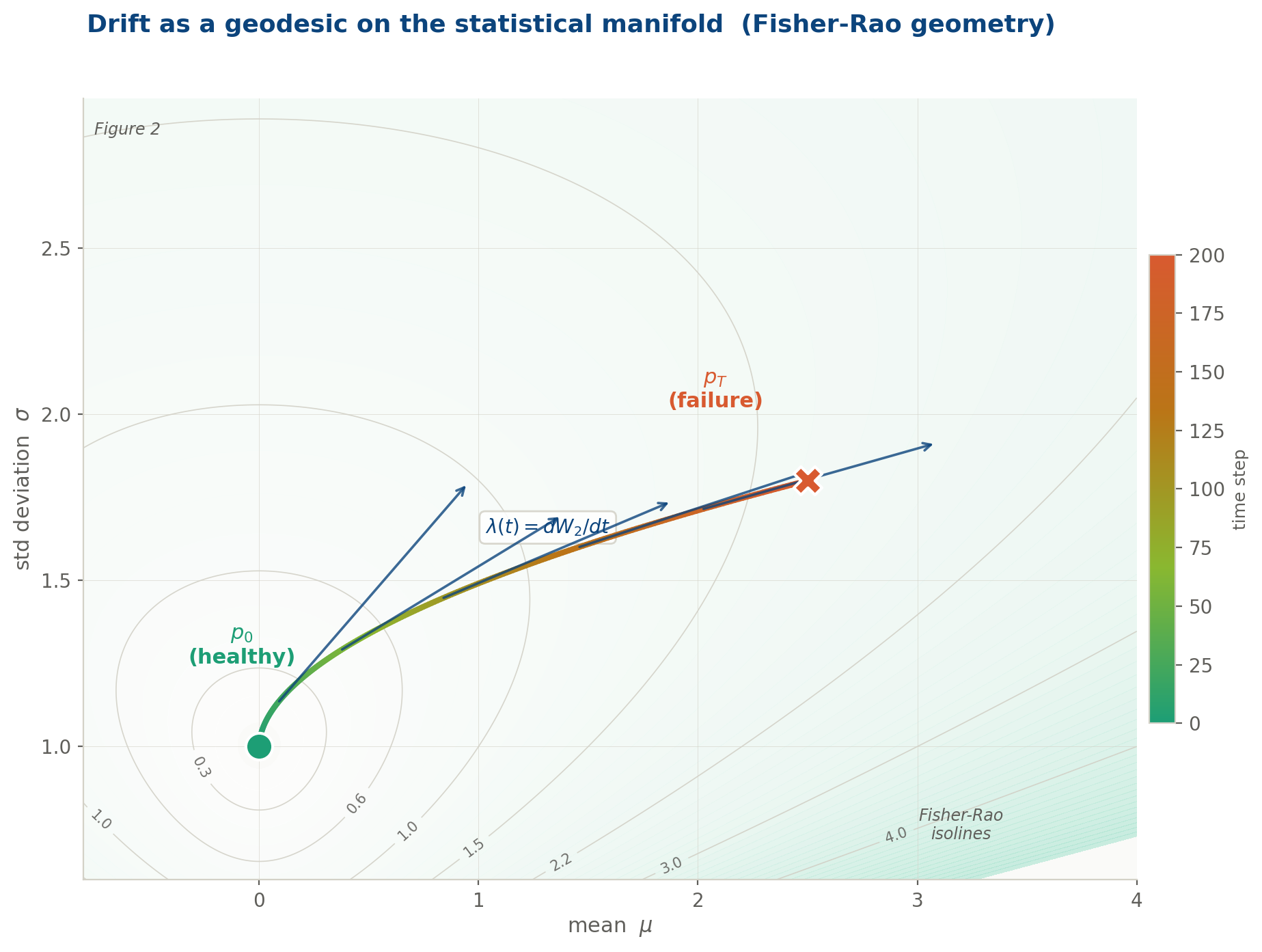
The drift trajectory plotted directly in (μ, σ) parameter space: the statistical manifold of the Gaussian family. Colour encodes time, from teal (healthy) through amber to rose (failure). Contour lines are Fisher-Rao isolines: each line is a set of distributions at equal statistical distinguishability from p₀. The trajectory accelerates as it moves into regions of higher curvature, where the geometry of distinguishability amplifies the apparent speed of change. The velocity arrows confirm what the curvature predicts: the process is not just moving, it is accelerating into unfamiliar distributional territory.
Two geometries, one phenomenon
At this point the post must be honest about something that is easy to elide.
W₂ and the Fisher-Rao metric are not the same thing. They live on different mathematical spaces and measure different aspects of distributional change.
W₂ lives on P₂(ℝ), the space of all probability measures with finite second moment. It is non-parametric: it sees the full shape of any distribution, not just the parameters of a assumed family. Its geodesics are mass interpolations, the curves along which one distribution morphs into another at minimum transport cost.
The Fisher-Rao metric lives on a parametric statistical manifold: the manifold of a specific family (Gaussian, here). It cannot see distributions outside that family. Its geodesics are paths through parameter space. Its distances are measured in units of statistical distinguishability: how many observations would a statistician need, on average, to tell these two distributions apart?
Both metrics penalise mean drift and variance drift. But Fisher-Rao penalises variance drift by √2 more, and normalises both by σ². The practical consequence is exact and important: when a process drifts primarily in its variance: widening, becoming erratic, without shifting its mean. The Fisher-Rao metric detects it earlier and amplifies the signal more strongly than W₂ does.
This is not a corner case. Variance drift (spreading tails, increasing dispersion, the process becoming less and less predictable) is among the most common and most dangerous modes of organisational failure. It is the mode that threshold-based controls miss longest, because the mean remains in bounds while the tails quietly thicken. The geometry that sees it earliest is Fisher-Rao.
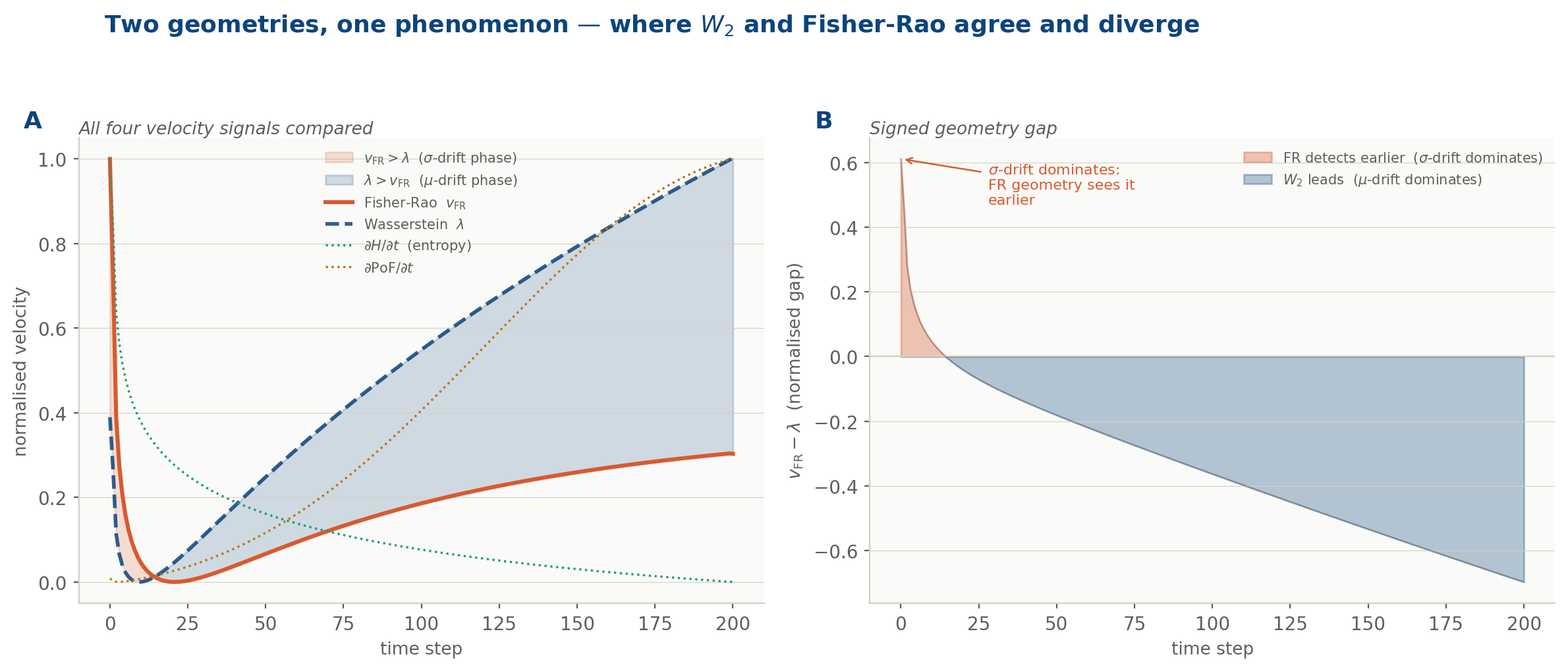
Panel A: all four velocity signals compared: Fisher-Rao v_FR (rose), Wasserstein λ (navy dashed), entropy gradient dH/dt (teal dotted), PoF gradient (amber dotted).
Panel B: the signed geometry gap. The rose region is where σ-drift dominates and Fisher-Rao detects the acceleration earlier. The navy region is where μ-drift dominates and W₂ leads. The two geometries agree on the presence of drift; they disagree on when it becomes dangerous.
What the five instruments were measuring
The series built five instruments. Each was introduced with its own mathematical framework, its own notation, its own motivating intuition. The deeper truth, the one visible only from the height of this post, is that all five were measuring the same geometric object from a different angle. There is a single identity that unifies them. For any smooth instrument Φ, its rate of change over time equals the inner product of its gradient with the drift vector λ, measured in the Fisher-Rao geometry.
Shannon entropy sees variance drift and spreading tails, but is blind to mean drift toward a threshold. Bayesian PoF sees exactly that mean drift, but misses variance widening away from the threshold. TSI reads connectivity changes and the emergence of multimodality, but cannot see unimodal drift or scale changes. CFI catches drift as it amplifies at structural chokepoints, but misses isotropic, structureless drift that flows through the graph uniformly. BOCPD detects discontinuities in drift, but is silent during smooth, continuous travel.
No single instrument covers the full object. Each covers a projection. Together, they span a larger subspace: but not the whole manifold.
Why entropy only sees variance drift
It is worth demonstrating this once, so the claim moves from asserted to proved, but without the full algebraic machinery.
Shannon entropy for a Gaussian depends only on the standard deviation: H = ln σ + const. Its gradient in parameter space points entirely in the σ direction and has zero component in the μ direction. Entropy is, in the most literal sense, blind to mean drift. It cannot see whether the process is shifting toward a threshold; it only sees whether the distribution is spreading or contracting.
The projection identity: that each instrument’s time-derivative equals the inner product of its gradient with the drift vector, in the Fisher-Rao geometry: confirms this precisely. When you compute the natural gradient of entropy (the Riemannian gradient, which weights directions by the Fisher information), you find it points only along the σ-axis. The inner product with the full drift vector λ = (dμ/dt, dσ/dt) then recovers exactly dσ/dt / σ: which is dH/dt. The dμ/dt term vanishes entirely.
So, entropy is a projection of λ onto the variance axis of the manifold. The full formal derivation, with matrix algebra, is in the appendix for readers who want it.
BOCPD: the instrument that catches jumps in λ, not λ itself
The fifth instrument deserves its own section, because it is qualitatively different from the other four: and understanding why reveals something fundamental about the limits of all projection-based monitoring.
BOCPD (Bayesian Online Changepoint Detection) does not monitor the level of drift. It monitors changes in the level of drift: discontinuities, regime shifts, moments when the process jumps from one distributional mode to another. The underlying model assumes that within any regime observations are exchangeable, and assigns at each time step a posterior probability that a new regime has just begun. Run length: the time elapsed since the last changepoint: accumulates evidence; when the evidence against the current run becomes strong enough, the detector fires.
But BOCPD has a structural blind spot that follows directly from its formulation: it is silent during smooth, continuous drift. While a process is travelling along a geodesic: while λ is positive but constant, while the distribution is migrating steadily away from baseline: the run-length posterior is long and stable. No changepoint is declared. The hazard signal remains flat. The drift is invisible to this instrument.
This is not a flaw. It is the consequence of BOCPD’s projection angle. It catches the discontinuity in λ, not λ itself.
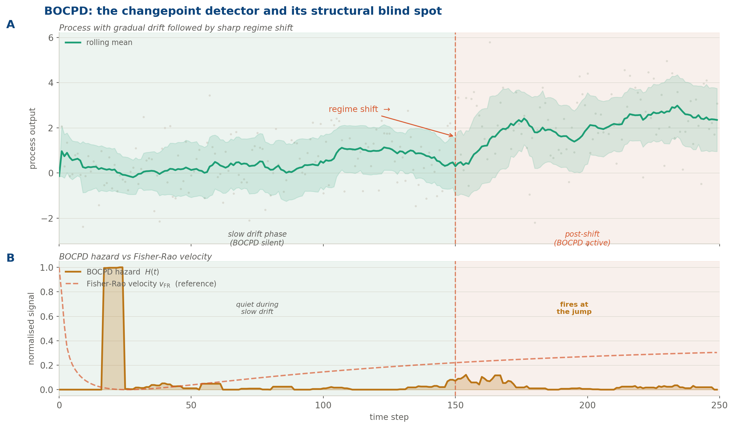
A two-phase process: gradual drift (0–150) followed by a sharp regime shift (at t = 150). Panel A shows the raw process, rolling mean, and ±1σ band. Panel B overlays the BOCPD hazard signal (amber) against the Fisher-Rao velocity (rose dashed). BOCPD is quiet during the slow drift phase: its projection angle simply cannot see smooth distributional travel. It fires decisively at the discontinuity. The Fisher-Rao velocity, by contrast, is elevated throughout the drift phase and would have flagged the departure from baseline long before the jump.
The Carillion case. Revisited
Before stating the unification abstractly, it is worth grounding it in the case that haunted this series from the beginning.
Carillion PLC: the UK construction and facilities management group that collapsed in January 2018 with £7 billion in liabilities and a pension deficit of £2.6 billion: was not a company that failed suddenly. Its audited accounts showed, in retrospect, a distributional trajectory that began diverging from sector peers around 2014. The patterns were there: revenue recognition policies that were shifting the distribution of reported cash flows toward the optimistic tail; debt-service coverage ratios whose variance was increasing quarter by quarter even as the mean remained technically within covenant; a dependency structure across subsidiaries whose cascade failure index was rising without triggering any single threshold.
Five instruments. Five partial projections. None declared failure. And yet, in the geometric language of this post: λ(t) > 0 from at least 2015. The distribution governing Carillion was moving. The dashboards were green. The trajectory was not.
Applied retrospectively, the five instruments tell a story: but each tells only a fragment of it, and only from its own angle. By 2014, the entropy signal was already climbing. The distributions of reported cash flows were spreading, their variance widening quarter by quarter, the process becoming less and less predictable even as the reported means stayed respectable. The PoF instruments saw nothing: the mean of every key ratio remained above its covenant floor, the threshold unthreatened, the alarm unmoved. By 2016 the topology had changed: the subsidiary dependency graph, which had previously formed a single connected cluster, was beginning to fragment, components drifting apart in a way that persistent homology would have caught and that no ratio-based test was looking for. The cascade failure index was rising in parallel, concentrating risk at a shrinking number of intercompany loan chokepoints: structural pressure building invisibly at the joints. And through all of it, from 2014 to the autumn of 2017, BOCPD was silent. There was no discontinuity to detect.
The direct Fisher-Rao velocity, estimated from the joint distribution of financial ratios across reporting periods, would have been non-zero and accelerating from 2015. Not because any single metric had breached a threshold. Because the distribution was moving: steadily, at an increasing speed, in the direction of failure.
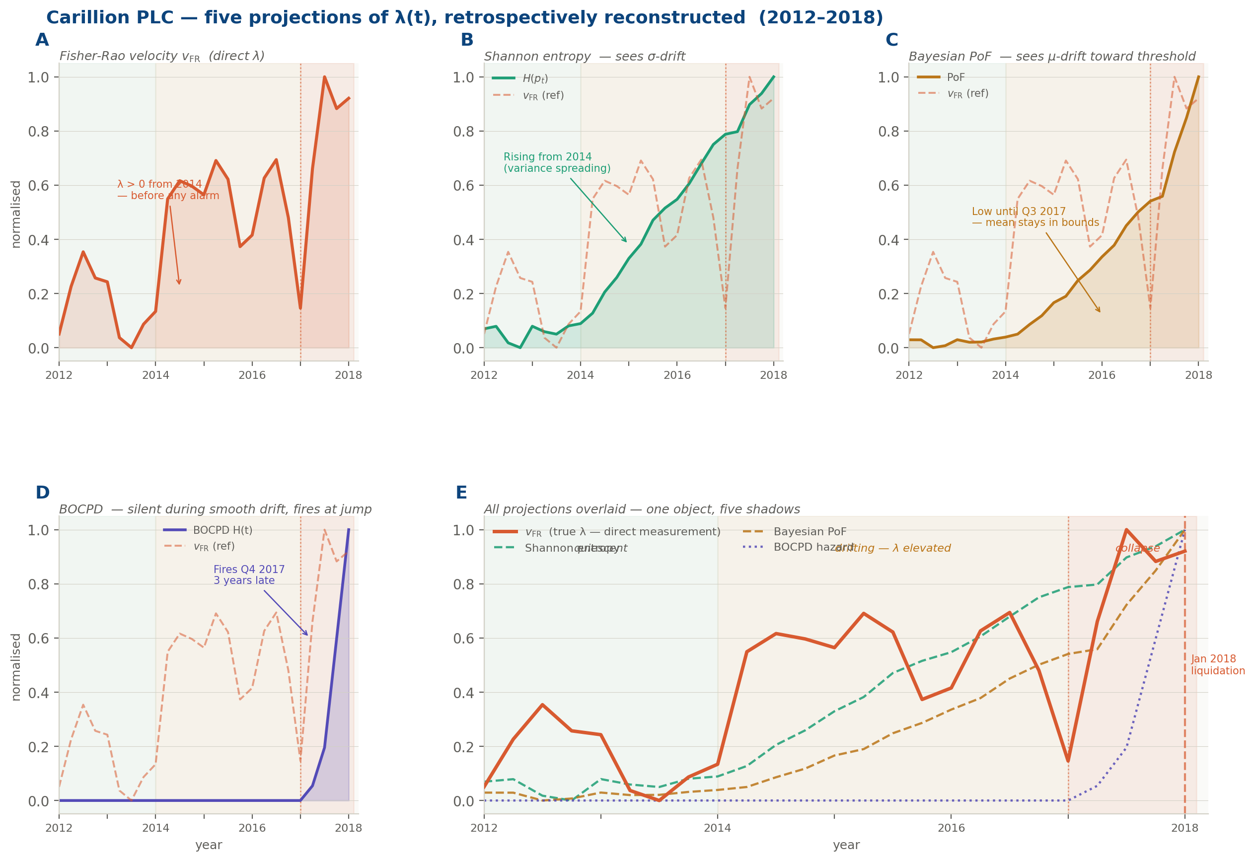
etrospective reconstruction of the five projection instruments applied to Carillion’s distributional trajectory (2012–2018). Panel A: the Fisher-Rao velocity: the direct λ(t): rising from 2014, three years before any public alarm. Panels B–D: Shannon entropy (detects σ-drift from 2014), Bayesian PoF (low until Q3 2017, because the mean stayed in bounds), and BOCPD (silent through the entire drift phase, firing only at the discontinuity in Q4 2017). Panel E: all signals overlaid. One geometric object.
Unification
The five instruments are not five competing methods. They are five projections of one geometric object.
Each instrument’s time-derivative equals the inner product of its gradient with the full drift vector: which means each one sees only the component of drift that falls along its own axis, and is blind to the rest. Five observed signals. Five angles. One vector.
The audit function, fully realised, is not a collection of methods. It is a single measurement: how fast is this organisation moving away from where it should be: and in which direction?
Direction is as important as speed. A process whose mean is drifting toward a threshold is a different danger from a process whose variance is expanding symmetrically.
The five instruments each see one direction. The Fisher-Rao velocity sees the speed. What is needed: and what no current audit toolkit provides: is the full velocity vector: magnitude and direction, measured directly on the manifold, without projection.
Drift in AI systems: the same manifold, a different domain
There is a reason this framework matters beyond enterprise audit.
The phenomenon of distributional shift in deployed machine learning systems is, mathematically, the identical object described above. A model trained on p_train and deployed into a world governed by p_t is experiencing a Wasserstein trajectory. Its predictions degrade because p_t has drifted away from p_train along the statistical manifold: not because the model is wrong, but because the ground has moved under it.
The ML monitoring field has independently developed its own set of projection instruments:
PSI, the Population Stability Index, computes a discretised KL divergence between the reference and current distributions: structurally, it is doing what Bayesian PoF does in the audit context, catching threshold-directed mass shift. CUSUM on prediction error accumulates deviations sequentially, making it the ML equivalent of BOCPD
Each of these instruments was developed independently, in a different community, motivated by different operational concerns. None was designed as a projection of a geometric object. Yet that is precisely what each one is. The convergence has a single name: λ. The drift velocity of a pharmaceutical process, a financial control environment, and a production neural network are all derivatives of the same Wasserstein trajectory. The same object. The same manifold. The same geometry.
The question: in every domain: is the same: how fast, and in which direction?
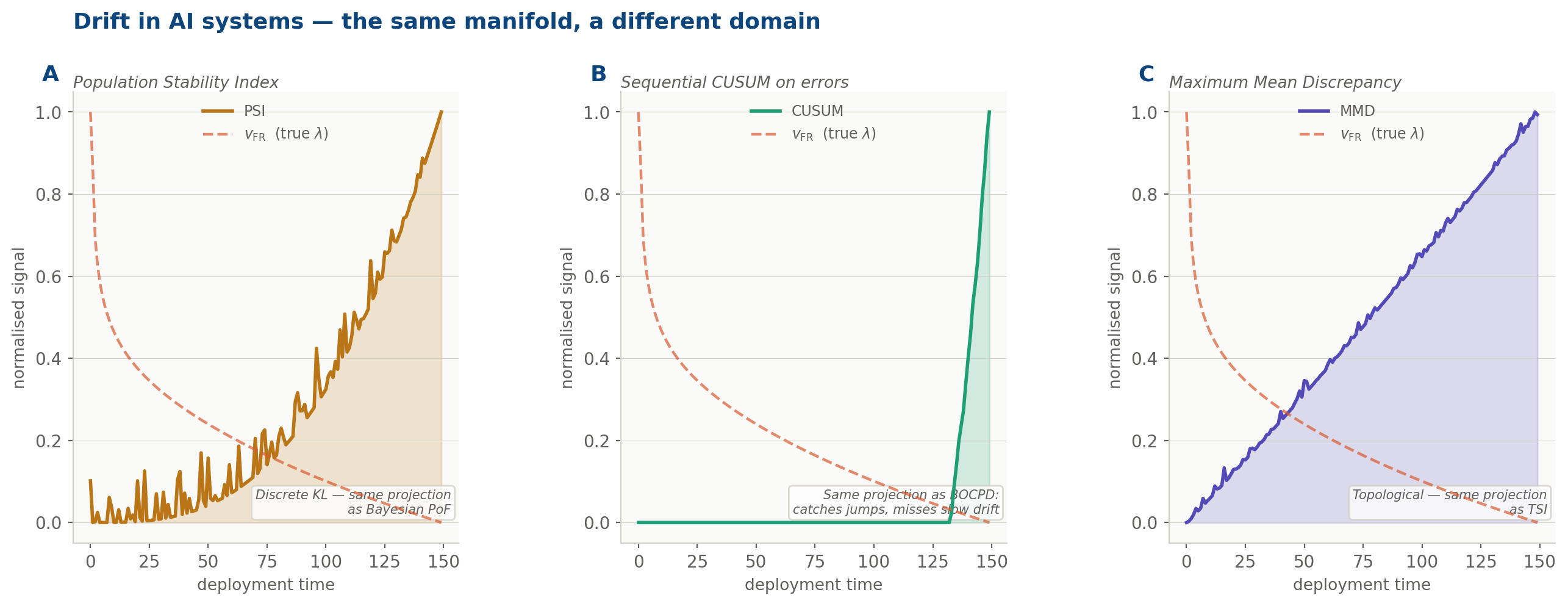
The three canonical ML drift detectors (PSI, CUSUM, MMD) overlaid against the Fisher-Rao velocity of the same drifting process. Each captures a different projection of λ. None captures the full object. The rose dashed line: v_FR: is what all three are approximating, from their respective angles.
What would direct measurement look like?
The five audit instruments and their ML counterparts are projections because direct measurement of λ requires estimating the Fisher-Rao velocity from streaming data, without assuming a parametric family, in real time. This is technically hard but not impossible. Three paths exist, each with a known computational profile.
Score-matching estimators. The Fisher information can be estimated from data without knowing the parametric form of the distribution, by estimating the score function: the gradient of the log-density. The score can be approximated by kernel methods or by small neural networks (the same architecture used in diffusion models). Practical cost: a sliding window of roughly 300–500 observations is sufficient for a stable univariate estimate.
Stein operators. The kernelised Stein discrepancy approximates the Fisher-Rao distance using only samples and a kernel function, without any density estimation. It achieves accuracy proportional to 1/√n: meaning 500 samples gives roughly ±0.045 on a normalised scale. Practical cost: quadratic in window size, tractable up to around 2,000 observations; Nyström approximation with 50–100 inducing points reduces this to near-linear, adequate for audit cadences of minutes to hours.
Wasserstein gradient flows. For parametric families, the drift velocity can be tracked directly via the natural gradient: the same object used in natural gradient descent and online expectation-maximisation. The Fisher matrix can be updated incrementally with rank-1 corrections, costing d² per observation rather than d³ per batch. Practical cost: the lightest of the three paths; fully online, suitable for high-frequency streaming data.
The practical upshot: for a process with up to 20 features, arriving at batch cadences of minutes or longer, all three paths are computationally feasible today using standard Python libraries. The bottleneck is not computation. It is the absence of an organisational decision to treat distributional drift as the primary audit observable: rather than a collection of ratio-based alarms that approximate it from different angles.
A reference implementation of the score-matching estimator for audit monitoring is in preparation for the next post in this series.
Next Quarter
We now came to an end of this alternative track which tried to provide an alternative to traditional Auditing getting inspirations from several mathematical techniques. The resulting direction deserves a framed research line which I would, if possible, address separately.
It is otherwise time to wait for a quarter shift for the topic I would explore during Q2/2026 - But I won’t reveal it now. Just be patient for two more weeks.